脈衝響應 Impulse Response

我們常看到脈衝響應  , 頻率響應, 其實都是在指 Transfer function !!

下面參考
http://translate.google.com.tw/translate?hl=zh-TW&sl=en&tl=zh-TW&u=http%3A%2F%2Fen.wikibooks.org%2Fwiki%2FControl_Systems%2FTransfer_Functions


Transfer Functions
傳遞函數的系統的輸入輸出系統的比例，考慮到其初始條件為零拉普拉斯域。
A Transfer Function is the ratio of the output of a system to the input of a system, in the Laplace domain considering its initial conditions to be zero.

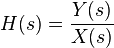
如果我們有一個X（S），和一個輸出函數Y（S）輸入功能，我們定義傳遞函數H（S）： If we have an input function of X(s) , and an output function Y(s) , we define the transfer function H(s) to be:



讀者閱讀電路理論書，將其識別為電路的脈衝響應的拉普拉斯變換的傳遞函數。 Readers who have read the Circuit Theory book will recognize the transfer function as being the Laplace transform of a circuit's impulse response.

脈衝響應 Impulse Response (in time domain)

為了便於比較，我們會考慮到上面的輸入 /輸出關係，相當於時域。
For comparison, we will consider the time-domain equivalent to the above input/output relationship.

在時域，我們通常指輸入到X（T）系統，系統的輸出為y（T）。

In the time domain, we generally denote the input to a system as x(t) , and the output of the system as y(t) .

輸入和輸出之間的關係表示為脈衝響應，H（T） 。The relationship between the input and the output is denoted as the impulse response , h(t) .

作為其輸入輸出系統之間的關係，我們定義的脈衝響應。

We define the impulse response as being the relationship between the system output to its input.

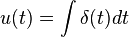
我們可以用下面的公式定義的脈衝響應：
We can use the following equation to define the impulse response:

脈衝函數  Impulse Function

脈衝函數 ，δ表示（t）是一個特殊的函數分段定義如下：

The Impulse Function , denoted with δ (t) is a special function defined piece-wise as follows:




脈衝函數也被稱為delta函數 ，因為它是用小寫希臘字母δ表示。
The impulse function is also known as the delta function because it's denoted with the Greek lower-case letter δ. delta函數通常是圖形趨於無窮大的箭頭，如下所示：
The delta function is typically graphed as an arrow towards infinity, as shown below:

它是繪製一個箭頭，因為它是在任何其他的圖形方法在無窮大的單點難以顯現。
It is drawn as an arrow because it is difficult to show a single point at infinity in any other graphing method.

請注意箭頭只存在於位置0，不存在任何其他的時間t。

Notice how the arrow only exists at location 0, and does not exist for any other time t .

衝激函數與固定的時間，就像任何其他功能的變化。

The delta function works with regular time shifts just like any other function.

例如，我們可以圖形的函數δ（T - N）的轉移函數δ（T）的權利，因此，

For instance, we can graph the function δ (t - N) by shifting the function δ (t) to the right, as such:

的衝動功能的檢查表明，它是有關單位階躍函數如下： An examination of the impulse function will show that it is related to the unit-step function as follows:

和 and

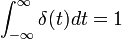
脈衝函數沒有定義點 t = 0，但總是脈衝響應必須滿足以下條件，否則它不是一個真正的脈衝函數： The impulse function is not defined at point t = 0 , but the impulse response must always satisfy the following condition, or else it is not a true impulse function:

脈衝輸入系統的響應稱為脈衝響應。

The response of a system to an impulse input is called the impulse response .

現在，脈衝函數的拉氏變換，我們採取的單位階躍函數，這意味著我們乘以單位階躍函數由S變換的導數： Now, to get the Laplace Transform of the impulse function, we take the derivative of the unit step function, which means we multiply the transform of the unit step function by s:

這一結果可以驗證在轉換表的附錄 。 This result can be verified in the transform tables in The Appendix .

頻率響應 Frequency Response

頻率響應是類似的傳遞函數，除了它是複雜的傅立葉域，而不是拉普拉斯域系統的輸出和輸入之間的關係。The Frequency Response is similar to the Transfer function, except that it is the relationship between the system output and input in the complex Fourier Domain, not the Laplace domain. 我們可以從傳遞函數的頻率響應，通過使用以下變量的變化： We can obtain the frequency response from the transfer function, by using the following change of variables:

S = jω s = j ω

頻率響應Frequency Response

該系統的頻率響應是關係到其輸入系統的輸出，在Fourier域表示。 The frequency response of a system is the relationship of the system's output to its input, represented in the Fourier Domain.

由於頻率響應和傳遞函數等密切相關，通常只有一個是有史以來計算，其他是由簡單的變量替換獲得。Because the frequency response and the transfer function are so closely related, typically only one is ever calculated, and the other is gained by simple variable substitution. 然而，儘管兩個表述之間的密切關係，他們都是有用的單獨，分別用於不同的目的。 However, despite the close relationship between the two representations, they are both useful individually, and are each used for different purposes.

階躍響應  Step Response

同樣的脈衝響應， 階躍響應系統的一個單位階躍函數作為輸入使用時，系統的輸出。

Similarly to the impulse response, the step response of a system is the output of the system when a unit step function is used as the input. 階躍響應是一種常見的的分析工具，以確定有關系統的某些指標。 The step response is a common analysis tool used to determine certain metrics about a system. 通常情況下，當一個新的系統設計，系統的階躍響應是要分析系統的第一個特點。 Typically, when a new system is designed, the step response of the system is the first characteristic of the system to be analyzed.

 卷積 Convolution

然而，脈衝響應不能被用來找到系統輸入輸出系統的傳遞函數相同的方式。

However, the impulse response cannot be used to find the system output from the system input in the same manner as the transfer function.

如果我們有系統的輸入和系統的脈衝響應，我們可以使用這種卷積運算計算系統的輸出：

If we have the system input and the impulse response of the system, we can calculate the system output using the convolution operation as such:

Y（T）= H（T）* X（T） y ( t ) = h ( t ) * x ( t )

其中“*”（星號）表示卷積運算。 Where " * " (asterisk) denotes the convolution operation. 卷積是一個複雜的乘法，集成和時移的組合。

Convolution is a complicated combination of multiplication, integration and time-shifting.

我們可以定義兩個函數，A（T）和B（T）以下之間的卷積：
We can define the convolution between two functions, a(t) and b(t) as the following:




（變量τ（希臘文頭）是一個集成的虛擬變量）。 (The variable τ (Greek tau) is a dummy variable for integration). 此操作可能難以執行。 This operation can be difficult to perform. 因此，許多人喜歡使用拉普拉斯變換（或其他變換）轉換成乘法運算的卷積運算，通過卷積定理 。 Therefore, many people prefer to use the Laplace Transform (or another transform) to convert the convolution operation into a multiplication operation, through the Convolution Theorem .

非時變系統響應 Time-Invariant System Response

如果有問題的系統時間不變，那麼系統的一般描述可以通過系統的脈衝響應的卷積積分和系統的輸入被替換。
If the system in question is time-invariant, then the general description of the system can be replaced by a convolution integral of the system's impulse response and the system input.

我們可以調用的一個系統的卷積描述，並定義如下：

We can call this the convolution description of a system, and define it below:

卷積定理 Convolution Theorem

這種系統的輸出的解決方法是相當乏味，其實如果你想解決多種輸入信號系統，它可以浪費了大量的時間。 This method of solving for the output of a system is quite tedious, and in fact it can waste a large amount of time if you want to solve a system for a variety of input signals. 幸運的是，拉普拉斯變換有一個特殊的屬性，稱為卷積定理 ，卷積容易操作： Luckily, the Laplace transform has a special property, called the Convolution Theorem , that makes the operation of convolution easier:


卷積定理可使用下列公式表示： The Convolution Theorem can be expressed using the following equations:

這也可以作為一個很好的例子二重性的財產。 This also serves as a good example of the property of Duality .

使用傳遞函數  Using the Transfer Function

傳遞函數完全描述一個控制系統。 The Transfer Function fully describes a control system. 秩序，類型和頻率響應都可以從這個特定的功能。 The Order, Type and Frequency response can all be taken from this specific function. Nyquist和Bode圖可以得出，從開環傳遞函數。 Nyquist and Bode plots can be drawn from the open loop Transfer Function. 這些圖顯示了系統的穩定性，當環路關閉。 These plots show the stability of the system when the loop is closed. 使用的傳遞函數的分母，稱為特徵方程可以推導出該系統的根。 Using the denominator of the transfer function, called the characteristic equation the roots of the system can be derived.

對於所有這些原因，並更多的傳遞函數是經典控制系統的一個重要方面。 For all these reasons and more, the Transfer function is an important aspect of classical control systems. 讓我們開始定義： Let's start out with the definition:


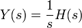
如果複雜的拉普拉斯變量s，那麼我們一般記為G（s）或H（S）系統的傳遞函數。 If the complex Laplace variable is s , then we generally denote the transfer function of a system as either G(s) or H(s) . 如果系統的輸入是X（S），系統輸出Y（S），然後傳遞函數可以這樣定義： If the system input is X(s) , and the system output is Y(s) , then the transfer function can be defined as such:

如果我們知道輸入到一個給定的的系統，我們有系統的傳遞函數，我們可以解決系統的輸出乘以： If we know the input to a given system, and we have the transfer function of the system, we can solve for the system output by multiplying:

[傳輸功能說明] [Transfer Function Description]

Y（S）= H（S）X（S） Y ( s ) = H ( s ) X ( s )

例子：脈衝響應  Example: Impulse Response

從拉普拉斯變換表中，我們知道，拉普拉斯變換，脈衝函數δ（T）是： From a Laplace transform table, we know that the Laplace transform of the impulse function, δ (t) is:

所以，當我們插入我們的輸入，輸出和傳遞函數之間的關係，這個結果，我們得到： So, when we plug this result into our relationship between the input, output, and transfer function, we get:

Y（S）= X（S）H（S） Y ( s ) = X ( s ) H ( s )

（1）Y（S）= H（S） Y ( s ) = (1) H ( s )

Y（S）= H（S） Y ( s ) = H ( s )

換言之，“脈衝響應”系統的輸出，當我們輸入一個脈衝函數。 In other words, the "impulse response" is the output of the system when we input an impulse function.

 例子：階躍響應 Example: Step Response

從拉普拉斯變換表中，我們還可以看到，單位階躍函數的變換，U（T）是： From the Laplace Transform table, we can also see that the transform of the unit step function, u(t) is given by:

插入到我們的傳遞函數的關係，結果給了我們： Plugging that result into our relation for the transfer function gives us:

Y（S）= X（S）H（S） Y ( s ) = X ( s ) H ( s )

我們可以看到，階躍響應僅僅是由 S分為脈衝響應。 And we can see that the step response is simply the impulse response divided by s .

 例子：MATLAB階躍響應  Example: MATLAB Step Response

使用MATLAB找到以下傳遞函數的階躍響應： Use MATLAB to find the step response of the following transfer function:

我們可以分離出來，這樣我們的分子和分母多項式： We can separate out our numerator and denominator polynomials as such:

NUM = [79 916 1000; num = [79 916 1000];
書房 = [1 30 300 1000 0]; den = [1 30 300 1000 0];
SYS = TF（NUM，DEN）; sys = tf(num, den);

現在，我們可以從我們的階躍響應，階躍函數和情節從1到10秒的時間： Now, we can get our step response from the step function, and plot it for time from 1 to 10 seconds:

T = 1:0.001:10; T = 1:0.001:10;
（SYS，T），步; step(sys, T);